Bouncing Ball

In this tutorial I will show you how to create a simple 2D bouncing ball simulation in Excel. For those who know Mechanics, we'll be looking at the Increamental/Numerical Method. This is where you have an initial value and calculate the change per frame. For this model the values we need are an initial position, velocity and an acceleration.

The starting position for the ball is -5 meters horizontal and 5 meters above the ground. A small horizontal velocity so the ball move slowly across. For the acceration the gravitial constant of 9.81 has been set, and as that for goes down it's set to minus.

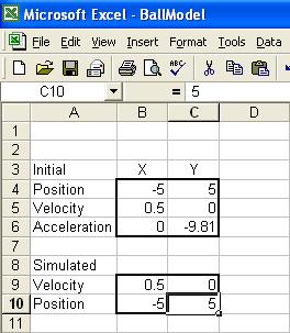
This is where we are going to store the values calculated each frame, the new velocity and the new position. Now to setup the macro, first we need some control values and two buttons Run and Reset.

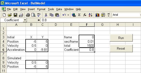Cell 'frame' is the number of the current frame, 'sec/frame', is how much a frame is worth in seconds for the calculation you might want to play about with this depending on the speed of the machine. 'total' is the end frame, 'Coefficient' is to do with friction and collision, put basicly it is the percentage of the energy thats left after a collision. Now last time we refered to each cell via absolute methods, "A1", "B1", etc. This time we'll give each cells names. The reason for names is once we've set up this model, we can move the cells around, but will still be linked via the name. Select cell B4 and in the dropdown box where it says B4 type 'Position' and press enter. You have now assigned the name 'Position' to Cell B4. Now select B5 and call it 'Velocity', B6 - 'Acceleration', B9 - 'SimVel' B10 - 'SimPos', F3 - 'frame', F5 - 'total' and F6 - 'Coefficient'. Now the buttons, control can also be given a name, one thats more useful that 'CommandButton1'. In design mode right click on a button and select properties.

In the properties window change the name and caption to 'Run', select the other button and change it to 'Reset'. While still in Design Mode double click on the Reset button and Enter the following: Private Sub Reset_Click() Range("frame") = 0 Range("SimVel")(1, 1) = Range("Velocity")(1, 1) Range("SimVel")(1, 2) = Range("Velocity")(1, 2) Range("SimPos")(1, 1) = Range("position")(1, 1) Range("SimPos")(1, 2) = Range("position")(1, 2) End Sub The above code resets the frame count and the simulation position and velocitys. Now if you double click on the Run button and Enter the following code: Private Sub Run_Click() Call Reset_Click While (Range("frame") < Range("total")) Range("SimVel")(1, 1) = Range("SimVel")(1, 1) + Range("Acceleration")(1, 1) * Range("frame")(2) Range("SimVel")(1, 2) = Range("SimVel")(1, 2) + Range("Acceleration")(1, 2) * Range("frame")(2) Range("SimPos")(1, 1) = Range("SimPos")(1, 1) + Range("SimVel")(1, 1) * Range("frame")(2) NewY = Range("SimPos")(1, 2) + Range("SimVel")(1, 2) * Range("frame")(2) If (NewY < 0) Then Range("SimVel")(1, 2) = -Range("SimVel")(1, 2) * Range("Coefficient") Range("SimPos")(1, 2) = Range("SimPos")(1, 2) + Range("SimVel")(1, 2) * Range("frame")(2) Else Range("SimPos")(1, 2) = NewY End If DoEvents Range("frame") = Range("frame") + 1 Wend End Sub

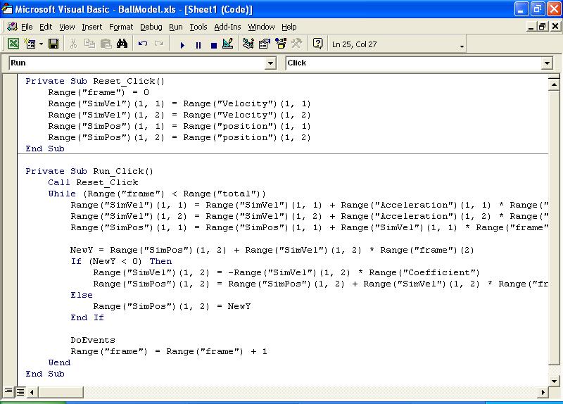Now the above code might look very scary, trust me it's not. This is what it does: First we Resets the simulation, then start the while loop. In the loop we calculate the new velocity and position and check that this position hasn't gone below the X-axis. if it has we invert the current velocity reduce it by the coefficient and re-calculate the position. Lastly we refresh the spreadsheet and increament 'frame'. Now thats the simulation done, you have now modeled a ball bouncing, all we need to do is display the results. Select the Simulated Position Values and click on the chart wizard. Select a scatter chart, click next and select the series tab. Now make the 'X Values' point to the X simulated position cell and do the equivlent for the 'Y Values'. If you click on finish you'll now have a chart. Almost finish, now Excel Chart auto size the scales of the axis, what we need to do is lock them down. Select the X-axis of the chart and double click it, this should bring up the format axis dialog, now select the scale tab.

Untick the top four checkboxes set min and max to -5 and 5, the major unit to 1 and the minor to 0.5. Max and min is the range of the axis, major unit is the increament of the scale, set to 1 it will go -5, -4, -3, etc. If you have a small chart you might want to increase this value. Minor unit is only seen if minor gridlines are displayed, this should be set as a fraction of Major unit, a half, fifth, etc. or just left as Auto. Now click Ok and do the same to the y-axis the only difference is the minimum can stay as zero, but remember to untick auto.

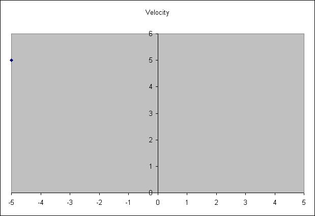
Hopefully your final chart will look like the across. Make sure you not in design mode and click run. You should now see the ball bounce. Things for you to try: Different initial settings Adding another ball Collision with the Y-Axis I'll be continuing the Excel theme and post another tutorial some time next week. Not sure what about yet. If you have any requests, leave it in the comments or PM on 3dbuzz.com and I'll see what I can do.

Cheers thing2k

Macros In Excel In recent thread at 3dbuzz, the poster of the thead ask about how to simulate a ball being dropped and bouncing on the floor. In my reply I included a Excel spreadsheet illustrating the simulation. In response to my reply I have been asked how I created the spreadsheet. So here I go... Macros are VBA scripts embedded in a Microsoft Office Document, they can be attached to cells, key commands and control objects. Here I only going to look at making a simple counter started by a buttons in Excel 2000. Open a new Excel document, right click on a menu and select Visual Basic. The icons left to right are: Run Macro, Record Marco, Security, Visual Basic Editor, Control Toolbox, Design Mode and Microsoft Script Editor. They are relatively self explanatory, so I'll just go over the ones we'll use, as we use them. Lets create a button, select Control Toolbox, then the button Icon in the Control Toolbox. If you notice, the Design Mode buttons are now selected and the a new toolbar has appeared. Only in design mode can you create and edit Controls. Now click somewhere on the sheet to create a button. To Change the buttons caption right click and highlight CommandButton Object and select Edit, and enter and caption you like. Now to get this button to do anything we need to start coding. Double click the button to bring up the VB editor. Now in the space type: Range("A1") = 0; while (Range("A1") <> Range("B1")) Range("A1") = Range("A1") + 1 DoEvents wend Going back to Excel, in cell B1 put in some large number like 123456789, exit design mode and click on your button. You should now see cell A1 quickly climb to the number you entered in cell B1. Now you've made a counter. Now to explain the code Range, is used to access a cells content. DoEvents, updates the current display. A few things you might what to try, create some forumlas that refer to cell A1. Create charts that refer to cell A1 and watch the dots move. I'll leave you now to play about with it. And I hope to be back soon with more you can do with macros in excel. thing2k

Hello

This is just a simple first post, just for me to get the hang of blogging (if that's actually a word).

I plan to use this blog as a place to post tutorials and experiences as I go through my last year at university. Also on the side I'm learning how to create homebrews for the PlayStation Portable. Not yet sure what I'm going to make in the end but I hope to produce a decent account of the steps along the way. I hope to post what I learn as I go.

I plan to update this a least once a week, but as the work load for uni increases, my post frequency will might(read:probably) drop.

Cheers

thing2k